Cement Slurry Rheological measurements

API sedimentation tests

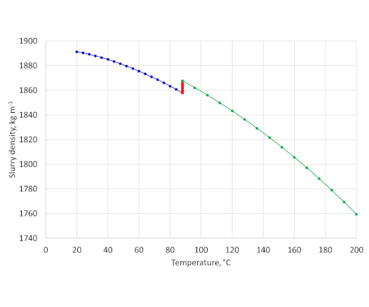
June 8, 2020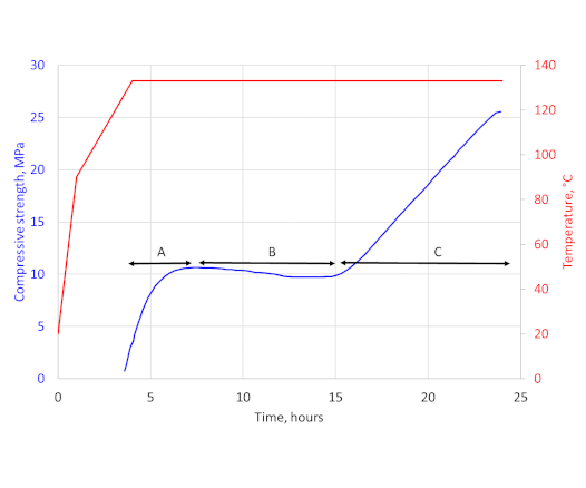

Compressive strength development at high temperature

December 10, 2020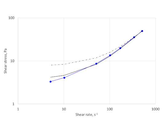

Errors in rheological measurements

API recommended practice RP10B-2 defines the correct procedures to determine the rheological parameters of cement slurries. However, incorrect procedures can still be seen in published work. The sections below discuss the most common errors observed.

Maximum recommended rotation speed

In both a peer reviewed article and a supplier data sheet rheological measurements included results at a viscometer rotational speed of 600 revolutions per minute (rpm). The highest recommended rotational speed in API RP10B-2 is 300 rpm, although readings at speeds > 300 rpm may be taken but after all other readings, including the gel strength measurements.

The limit on the maximum rotational speed while making rheological measurements on cement slurries is based on comparative testing between multiple laboratories (Beirute, R.M.: “API Revises Procedures to Measure Cement Slurry Rheology,” Oil & Gas Journal, (September 1, 1986) 84, No. 38, 36–38). The study found that there was better repeatability of measurements if the upper shear rate was limited to 511 s^-1. Note, that at that time there was only one bob and rotor geometry (R1B1) generally used, so 511 s^-1 corresponded to 300 rpm.

Ramp up and ramp down measurements

In the documents there was also no indication that the results presented were an average of readings taken ramping up and ramping down in shear rate, as required by API RP10B-2. Taking ramp up and ramp down readings can help indicate if the fluid has time dependent (thixotropic) properties or if the fluid is unstable. A possible presentation of rheological measurements is shown below. It follows the guidelines in API RP10B-2, 2^nd edition, April 2013.

	Reading
Rotational Speed (rpm)	Ramp-up	Ramp-down	Ratio	Average
3	8	5	1.6	6.5
6	9	7	1.29	8
30	18	16	1.13	17
60	27	26	1.04	26.5
100	39	39	1	39
200	69	70	0.99	69.5
300	97	-	-	97
Rheometer configuration	R1-B1-F1
Conditioning	Atmospheric pressure, 30 minutes at 50°C
Initial slurry temperature	50°C
Final slurry temperature	48°C

In this example, the ramp up and ramp down readings are close (<5 units) so there is no indication of sedimentation or gelation. Note that these observations are not a substitute for static gel strength measurements or sedimentation tests.

Model fitting - Bingham Model

The documents both fitted the date with the Bingham model:

τ = τ_y + μ_pɣ̇

Where τ is the shear stress at a shear rate ɣ̇. τ_y is the Bingham yield stress and μ_p is the plastic viscosity. When the shear stress, τ, is less than the Bingham yield stress there is no flow. Bingham plastic fluids are therefore shear thinning once the shear stress is greater than the yield stress.

Even though curve fitting is easy to do with spreadsheets there is still a tendency for people to use just two data points to fit the data, which was the case with the peer reviewed journal article (using 600 and 300 rpm data points). API RP 10B-2 clearly states that 2-point calculations should not be used.

As an example, I will use the average data points from the above table - I have converted the rpm and dial reading to shear rate (s^-1) and shear stress (Pa) for the following analysis. Data fitting for the Bingham model has been done using the built in linear regression function in Excel.

The results for the fit are shown in Figure 1.

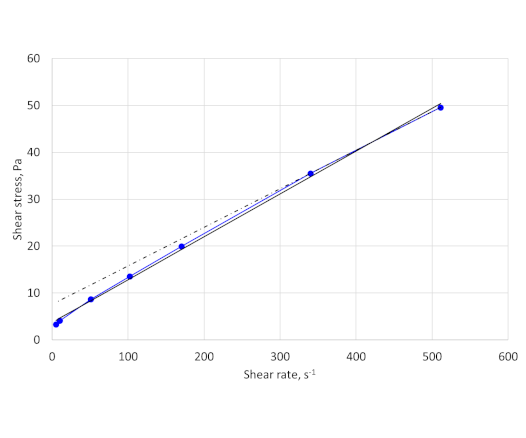
The curve fit using just the two data points at the highest shear rates does not match the data over the entire range and gives a yield stress value of 7.6 Pa. The curve fit using all the data points give a much better fit of the data over the entire range. The yield stress value is 3.7 Pa. The reading at 5.1 s^-1 (3 rpm) is 3.3 Pa.

In most cases fitting the data using all the data points will give a higher plastic viscosity and lower yield stress than using a two-point data fit at high shear rates. Exceptions will be fluids exhibiting dilatancy (shear thickening).

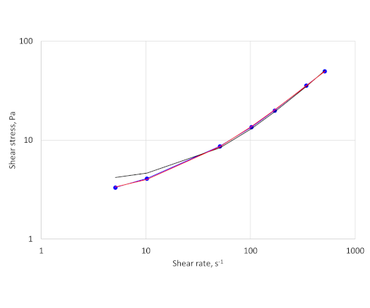
The differences between the fits and the actual data can be seen more clearly on a log-log (Figure 2). The fit using all 7 data points overestimates the low shear rate viscosity but is much closer to the data than the two-point fit.

Plotting the data on a log-log plot also shows that there are no signs of slippage at the wall, as the data points follow a smooth curve.

Model fitting – Herschel-Bulkley model

The Herschel-Bulkley model is a three-parameter model that combines power law and Bingham plastic behaviour.

τ = τ_y+ kγ̇ⁿ

Where k is the consistency index, and n is the power law index.

The Herschel-Bulkley model simplifies to the Bingham model (if n=1) and to the power law model with τ_y=0.

Microsoft Excel can also be used to fit the Herschel-Bulkley model to a set of data as follows:

Convert the rpm values and average dial readings to shear rate (s^-1) and shear stress (Pa) respectively.
Estimate a yield stress value, this can be from 0 to the shear stress determined at 3 rpm (5.1 s^-1).
Use this estimated yield stress to perform a linear regression on log((shear stress – estimated yield stress)/Pa) v log(shear rate/s^-1) to give n and k.
Calculate the sum of the squares of the differences between the data points and the calculated values.
The Excel solver function can then be used to determine the value of the yield stress, and the associated n and k values, that minimises the sum of the squares.

The best fit to the data above has:

τ_y=2.6 Pa, n=0.897, k=0.175 Pa.sⁿ

The fit is plotted in Figure 3:

HB Fit — Figure 3 The blue dots are the data points. The solid black line is the Bingham model fit using all 7 data points. The red line is the Herschel-Bulkley fit using all the data points.

There is a more detailed discussion of fitting rheological models to data of drilling and cementing fluids in:

Hans Joakim Skadsem and Arild Saasen, “Concentric cylinder viscometer flows of Herschel-Bulkley fluids”, Appl. Rheol. 2019; 29 (1):173–181.

This is an open access paper available at: https://doi.org/10.1515/arh-2019-0001